Timeline Like a Boss

Timeline Like a Boss!

Timelining allows a forensic analyst to examine a system at a granular level and can provide insight into what is going on at a certain point in time. Before an analyst engages in timeline analysis they should take a few things into account to avoid rabbit holes and be efficient in their analysis:

• Narrow scope of time as much as possible
• All commands should be run from an administrator prompt, or with sudo permissions

Filesystem Timeline Creation:

A file system timeline is a critical piece of evidence that gives great insight into actions that occurred on the filesystem. We will start on a Windows VM using Eric Zimmerman’s MFTECmd.exe. This tool takes an $MFT file and parses it into a body file. The preferred command is:

MFTECmd.exe -f [Path to MFT File] --body [Directory you want to output to] --bodyf [Name for file] -blf –bdl C: 

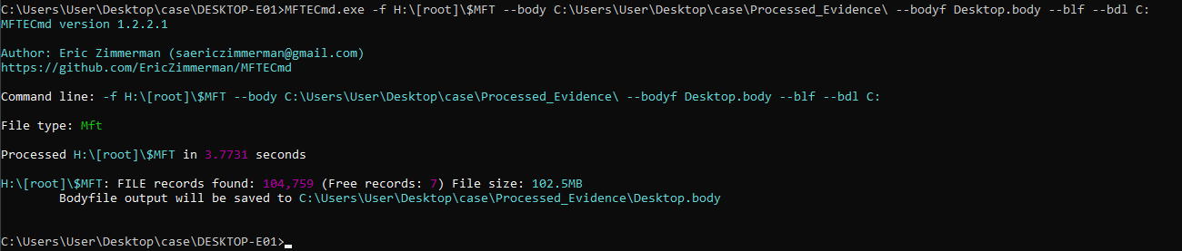
This command leaves us with a body file that we can ingest via various means. The preferred method is to take the body file over to a Linux system (WSL is also viable). Once on the Linux system we can use “mactime” to parse the body file into a CSV file. We can also use mactime to narrow our time scope if desired!

mactime -z [Time zone of the ANALYSIS VM (Should be UTC)] -y -d -b [path to body file]  [Time range, yyyy-mm-dd (Can be left blank)]  > [Path_to_output_File].csv 

Once mactime is complete you will be left with a csv file that you can analyze in any way you see fit!

Super Timeline Creation:

For our Super Timeline Generation we are going to use a SIFT VM. There are ways to generate a timeline in Windows but we will not cover them here, the preferred method will be via SIFT VM. Also keep in mind that we are generating a super timeline, not just a filesystem timeline and it typically is a significantly longer process.

Mounting VHDX in Linux (Optional):

We will briefly discuss how to mount VHDX files in Linux because other scenarios could make it necessary. However, we do not need to have the VHDX mounted in order to process it with Log2Timeline!

First we will use the virtualization tool “qemu-nbd” to mount the vhdx file. Before this we need to ensure that “nbd” kernel module is loaded and enabled for partition support.

 modprobe nbd max_part=16 

Next we can use qemu-nbd to connect the vhdx to the the NBD device.

qemu-hbd -c /dev/nbd0 [path to vhdx file] 

We will then us partprobe to inform the OS of the Partition table changes.

partprobe /dev/nbd0 

Finally let’s make a directory and mount the first partition.

mkdir /mnt/[name] 
mountwin /dev/nbd0p1 /mnt/[name] 

Now let’s check and make sure we can see files and folders!

ls /mnt/[name] 

Creating Supertimelines:

Log2Timeline uses Plaso as an engine to parse through artifacts and generate a timeline that we can then use to perform our analysis. While Plaso is made with python and is cross platform, the preferred way of running it is via docker. We will first cover setting up the docker image then the steps necessary to create a timeline. The below will pull the latest log2timeline image from docker hub and the second command will test to make sure everything is running as expected. Note that this will require internet connectivity!

docker pull log2timeline/plaso 
docker run log2timeline/plaso log2timeline.py --version 

Once we have our docker image we can begin working on timeline creations. All of our commands will have to be run through the docker container so we will be using the Docker syntax. Don’t worry it is not too bad and is much better than fighting dependencies!

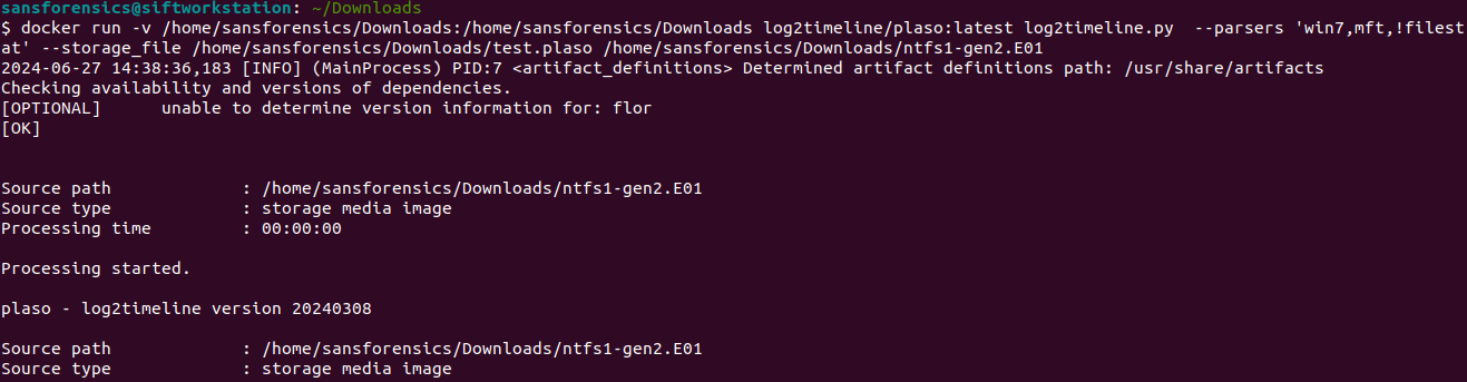
We will begin by parsing the vhdx image that we mounted previously. This command is long but I will do my best to break it down.

docker run –v /cases:/cases -v /mnt/[name of vhdx]:/mnt/[name of vhdx] log2timeline/plaso log2timeline.py --timezone [timezone of subject system] --parsers 'win7,!filestat' --storage_file /cases/triage/[output.plaso] [mount_point_of_Subject] 

Okay now we are going to take this in chunks:

• docker run –v /cases:/cases -v /mnt/[name of vhdx]:/mnt/[name of vhdx] log2timeline/plaso log2timeline.py
  • This portion starts the docker image and runs the log2timeline.py command within it.
  • It also binds the /cases directory in the sift vm to a /cases directory within the container
  • The next part of the command binds the directory where we mounted the vhdx file to the container
• ”–timezone [timezone of subject system] “
  • This portion needs to contain the timezone that the subject system is running. You can run “–timezone list” to get a list of timezones
• ”–parsers ‘win7,!filestat’”
  • This runs the win7 parsers and excludes the filestat parser. It is more efficient to exclude the filestat parser and add in the filesystem timeline separately, which we will show.
• ”–storage_file /cases/triage/[output.plaso] [mount_point_of_Subject]”
  • This directs log2timeline to parse all files in the mount point and store the output in the plaso database. If this completes successfully you should have a Plaso database ready for analysis. However, we promised to add in the filesystem timeline, which we will do now. We will highlight differences from the above command as they are very similar. Note that in the below screenshot since my image was small I processed $MFT with log2timeline as well. However below you will find details on how we would take an already generated body file and combine it with our timeline.

- docker run –v /cases:/cases log2timeline/plaso log2timeline.py --parsers 'mactime' --storage_file /cases/triage/[output.plaso] [path to bodyfile]  - docker run –v /cases:/cases log2timeline/plaso log2timeline.py 
- For this portion all the data we need should reside in the /cases directory (output.plaso and bodyfile), therefore that is the only directory that we need to bind to the container.  - "--parsers 'mactime'"
- This specifies that we want to use the mactime parser. - "--storage_file /cases/triage/[output.plaso] [path to bodyfile]"
- This tells log2timeline the plaso database that we want to add to and we also give it the path to the body file here. Our Plaso database is then ready to be analyzed!

Parsing for Analysis:

This next command is an even bigger monster but good news is that it is our last one!

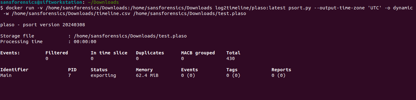
- docker run -v /cases:/cases log2timeline/plaso psort.py --output-time-zone 'UTC' -o dynamic -w [output csv file] [path to plaso database] "(((parser =='winevtx') and (timestamp_desc == 'Creation Time')) or (parser != 'winevtx')) and ( date > datetime('[Lower time bound]') AND date < datetime('[upper time bound]'))"

Now do not freak out. We are going to go over this, and some of the switches should be familiar at this point.

• docker run -v /cases:/cases log2timeline/plaso psort.py –output-time-zone ‘UTC’ -o dynamic -w [output csv file] [path to plaso database]
  • Here we are doing similar things in terms of binding our case directory to the container, but instead of running log2timeline, we are running psort.py to manipulate the data in our plaso database.
  • Next, we tell psort that we want the output time zone to be UTC.
  • Lastly, we are specifying where we would like the csv output file to be written and then specifying the plaso database to use.
• ”(((parser ==’winevtx’) and (timestamp_desc == ‘Creation Time’)) or (parser != ‘winevtx’)) and ( date > datetime(‘[Lower time bound]’) AND date < datetime(‘[upper time bound]’))”
  • This looks more intimidating than it is mostly because the syntax is not as friendly to the eyes. Essentially, Event logs have a Creation and a Modification event that will trigger(https://blog.fox-it.com/2019/06/04/export-corrupts-windows-event-log-files/). We are using psort to only show us events with a creation timestamp
  • Following this filter we are pulling all the other artifacts.
  • We are then giving and upper and lower bound in terms of time.

Now hopefully you have a CSV file that is ready for analysis however you see fit. The next section is purely extra and is for those of you who want to work on doing forensic at scale! If you do run into issues when converting to CSV remove the filters in the psort.py portion and see what you end up with.

Scaling Up with Timesketch!

Timeline analysis is a proven method for Incident response and Digital Forensics. However it can get overwhelming when you have more than a handful of systems, or even one system if the scope is large. This is where Timesketch comes into play (https://timesketch.org)! There are other guides for how to install Timesketch and the best implementations, this will not be covered here. I run Timesketch in a more tactical capacity via a docker container on my analysis VM.

When you open the Timesketch web UI you will be greeted with something similar to this. There is a legacy UI available but I personally prefer the new UI. Also note that the VM I am using has SANS lab data in it, but we will not be performing any in depth analysis to avoid copyright.

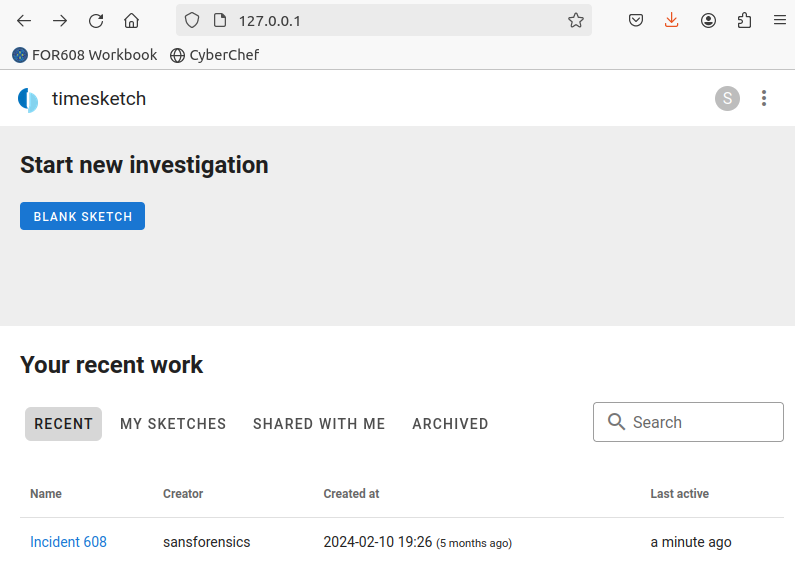
Listed at the bottom of the picture is where we see our “sketches”, sketches are the equivalent to a case and can hold multiple artifact types/sources. Think of them as the folder that your evidence files are in.

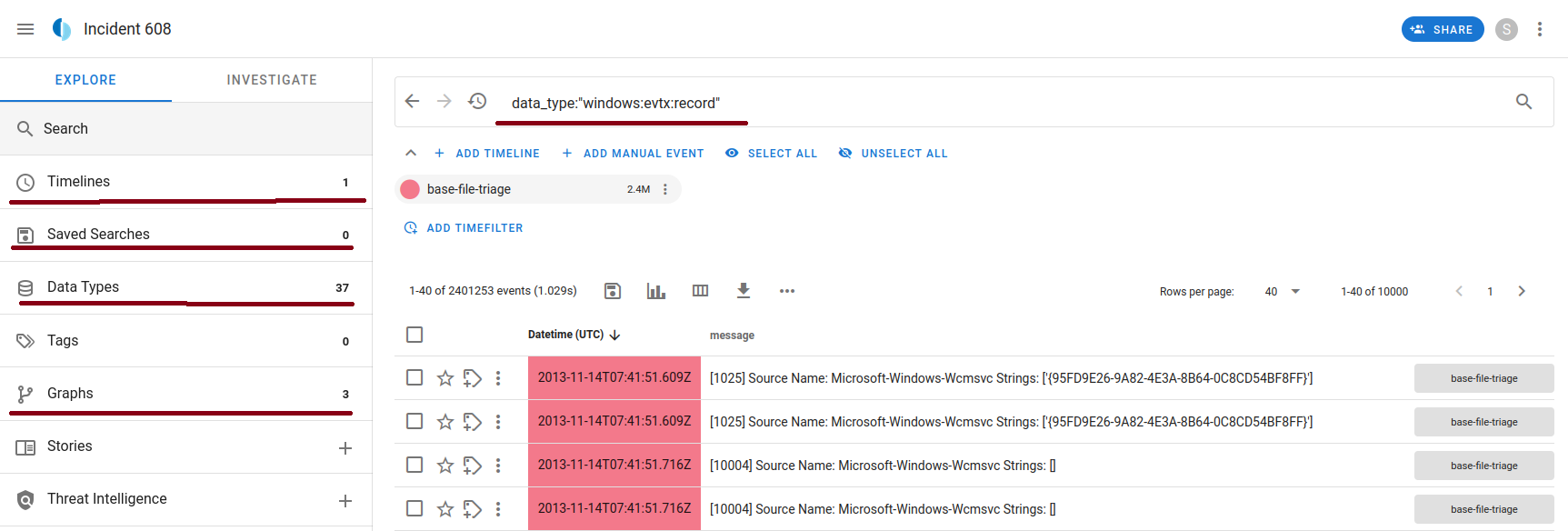
If we drill down into our sketch we will be presented with something similar to the above. There are a handful of tabs that as an analyst you must be aware of! Let’s discuss these in just a little bit of depth!

Timelines

Data Types

Search

Saved Searches

Graphs

Common Issues:

• I have seen issues where Log2Timeline is unable to parse multiple partitions and errors out. One easy fix is to mount the image in question and run Log2Timeline against the mount point instead. However it Should be able to handle most drive types.
• Understanding the time zones is important!!!